Raster vs. Vector

Vector is Corrector.

Object data model:

• generalization
• represent real things as locations and attributes
• objects = conceptualizations of real items
• concrete or abstract

{
    "type": "Feature",
    "geometry": {
        "type": "Point",
        "coordinates": [77.230004, 28.6947]
    },
    "properties": {
        "name": "Majnu ka Tilla",
        "type": "food joints",
        "rating": 4.5,
        "state": "Delhi",
        "country": "India"
    }
}

Restaurant Name	Coordinates	Food Type	Cost (1-5)	Hours	Capacity	Rating
Ama Restaurant	[77.2305, 28.6948]	Tibetan, Chinese	2	11AM-10PM	40	4.3
Dolma House	[77.2307, 28.6945]	Tibetan	2	10AM-9PM	25	4.4
AMA Cafe	[77.2306, 28.6947]	Cafe, Breakfast	3	8AM-9PM	30	4.6
Rigo Restaurant	[77.2304, 28.6946]	Korean, Japanese	3	12PM-10PM	35	4.2
Busan Korean	[77.2305, 28.6949]	Korean	4	12PM-11PM	45	4.5

Rester is faster, but vector is corrector.

Vector caclculations:

• re-projection is precise
• reliably stores:
• point overvations
• edges
• boundaries
• attributes stay reliable if joined properly

Raster is Faster.

Raster data model:

raster data model

Raster alignment:

• location, grid of values
• raster become difficult when comparing locations (10m cell size vs 15m cell size)
• need to decide which cells should overlap

Raster re-projection:

• introduces errors
• lossy data
• less precise than vector

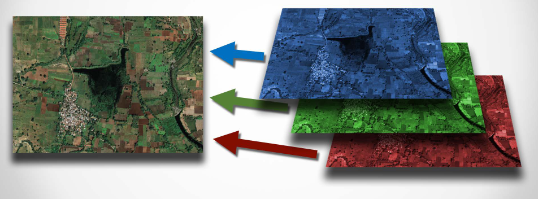
Multiband raster:

• rasters can be stacked to work with multiple rasters as if they're one.
• each "band" is a single raster.
• ex: represent data from different sensors captured at the same time.

Geodatabase Data Types

Summary Table of Concepts in Data Types and Management

Concept	Description	Examples/Details	Key Considerations
Data Types (General)	Categories defining how data is stored, grouped, and processed. Determine valid operations and storage efficiency.	Numbers, text strings, dates/times.	Crucial for operations (e.g., math on numbers, not text). Affects tools, queries, and programming.
Binary Interpretation	Data is stored as binary (0s/1s). Interpretation depends on data type.	Binary 1010100 = 84 (number) or T (text).	Incorrect data type leads to misinterpretation (e.g., 84 vs. T).
Integer Types	Whole numbers (no decimals). Subtypes vary by storage size and range.	Short Integer: -32,768 to 32,767 (16 bits). Long Integer: ±2 billion (32 bits).	Use short integers for small ranges (e.g., 0-90° slope) to save space.
Decimal Types	Real numbers with decimal precision. Floating-point numbers allow variable decimal placement.	Float (Single): ±10³⁸ (32 bits). Double: ±10³⁰⁸ (64 bits).	Use doubles for extreme precision/size. More storage and computational cost than integers.
Text Strings	Stores text or numbers treated as text (non-mathematical).	ZIP codes, categories (e.g., "A1", "100-MainSt").	ArcGIS file geodatabases lack length limits. Other systems may require length specs.
Null Values	Represents undefined/unknown data (distinct from zero).	Unpopulated fields, missing measurements.	Math with nulls returns nulls (e.g., 5 + null = null). Requires data cleanup.
Field Naming	Rules for naming fields to ensure clarity and compatibility.	Use camelCase or underscores; avoid spaces (e.g., SlopeDegrees or slope_deg).	Consistency and descriptiveness aid usability. Spaces may break database commands.

---

Key Takeaways:

• Storage Efficiency: Choose data types based on required range/precision (e.g., short vs. long integers).
• Operations: Data types enable/disallow operations (e.g., math on numbers, text concatenation).
• Null Handling: Nulls require special handling in calculations and analysis.
• Naming Conventions: Improve readability and system compatibility.

---

Vector attribute datasets

Data Joins & Relational Concepts: Real-World Examples

---

Core Concepts with Global Examples

1. Primary & Foreign Keys

Concept:

• Primary Key (PK): A unique identifier for records in a table (e.g., auto-generated IDs).
• Foreign Key (FK): A field in one table that references the primary key of another table.

Real-World Example:

Eiffel Tower Maintenance

• Landmarks Table (Primary Key: landmark_id):

  landmark_id	name	height_m
  101	Eiffel Tower	330

• Maintenance_Logs Table (Foreign Key: landmark_id):

  log_id	landmark_id	date
  201	101	2023-09-01

Yelp Restaurant Reviews

• Restaurants Table (PK: restaurant_id):

  restaurant_id	name
  301	Central Park Café

• Reviews Table (FK: restaurant_id):

  review_id	restaurant_id	rating
  401	301	4.5

Why It Works: Avoids duplicating restaurant details in every review.

---

2. Types of Joins

Concept: Linking tables based on shared attributes or location.

Table Join Example (Disney World)

Scenario: Linking ride locations to wait times.

• Rides Table (PK: ride_id):

  ride_id	name
  501	Space Mountain

• Wait_Times Table (FK: ride_id):

  time_id	ride_id	wait_minutes
  601	501	45

Spatial Join Example (Tokyo Subway)

Scenario: Counting subway stations per neighborhood.

• Subway_Stations (Points) ↔ Neighborhoods (Polygons).

---

3. ArcGIS Relates vs. Joins

Concept:

• Joins merge attributes into one table (1:1 or 1:many).
• Relates link tables dynamically without duplication (1:many, many:many).

Real-World Use Case:
Great Barrier Reef Monitoring

• Reef_Polygons (1 record per reef) ↔ Coral_Health (multiple health scores per reef).

Reef_ID	Reef_Name
701	Agincourt Reef

Health_ID	Reef_ID	Health_Score
801	701	8.5

Why Use a Relate?
Avoids duplicating reef geometry for each health score entry.

---

📊 Summary Table: Join Types & Use Cases

Concept	Example	Global Use Case
Primary Key	landmark_id for Eiffel Tower	Unique IDs for landmarks, users, products.
Foreign Key	restaurant_id in Yelp reviews	Linking reviews to businesses.
Spatial Join	Tokyo subway stations ↔ neighborhoods	Urban planning, disaster response.
Relate	Great Barrier Reef health data	Environmental monitoring, research.

---

Practical Exercise: Design a Tourism Database

Scenario: Machu Picchu Visitor Management
Task: Design tables to track visitors, tickets, and archaeological sites.